Multiple Random Gabor experiment

In this quick experiment we will be training an MNIST classifier using multiple RandomGabor layers.

Library importing

import numpy as np
import matplotlib.pyplot as plt
from einops import rearrange, repeat

import tensorflow as tf
from tensorflow.keras import layers
from tensorflow.keras.datasets import mnist

from flayers.layers import RandomGabor

Data loading

We will be using MNIST for a simple and quick test.

(X_train, Y_train), (X_test, Y_test) = mnist.load_data()

X_train = repeat(X_train, "b h w ->  b h w c", c=1)/255.0
X_test = repeat(X_test, "b h w ->  b h w c", c=1)/255.0

X_train.shape, Y_train.shape, X_test.shape, Y_test.shape

((60000, 28, 28, 1), (60000,), (10000, 28, 28, 1), (10000,))

Definition of simple model

model = tf.keras.Sequential([
    RandomGabor(n_gabors=4, size=20, input_shape=(28,28,1)),
    layers.MaxPool2D(2),
    RandomGabor(n_gabors=4, size=20),
    layers.MaxPool2D(2),
    RandomGabor(n_gabors=4, size=20),
    layers.MaxPool2D(2),
    layers.GlobalAveragePooling2D(),
    layers.Dense(10, activation="softmax")
])
model.compile(optimizer="adam",
              loss="sparse_categorical_crossentropy",
              metrics=["accuracy"])
model.summary()

2022-09-20 12:47:21.299667: I tensorflow/core/common_runtime/gpu/gpu_device.cc:1510] Created device /job:localhost/replica:0/task:0/device:GPU:0 with 5435 MB memory:  -> device: 0, name: NVIDIA GeForce GTX TITAN Black, pci bus id: 0000:83:00.0, compute capability: 3.5
2022-09-20 12:47:23.872491: I tensorflow/compiler/mlir/mlir_graph_optimization_pass.cc:185] None of the MLIR Optimization Passes are enabled (registered 2)
2022-09-20 12:47:24.116626: I tensorflow/core/util/cuda_solvers.cc:180] Creating CudaSolver handles for stream 0x5566d7fd5170

Model: "sequential"
_________________________________________________________________
Layer (type)                 Output Shape              Param #   
=================================================================
random_gabor_1 (RandomGabor) (None, 28, 28, 4)         1626      
_________________________________________________________________
max_pooling2d (MaxPooling2D) (None, 14, 14, 4)         0         
_________________________________________________________________
random_gabor_3 (RandomGabor) (None, 14, 14, 4)         1626      
_________________________________________________________________
max_pooling2d_1 (MaxPooling2 (None, 7, 7, 4)           0         
_________________________________________________________________
random_gabor_5 (RandomGabor) (None, 7, 7, 4)           1626      
_________________________________________________________________
max_pooling2d_2 (MaxPooling2 (None, 3, 3, 4)           0         
_________________________________________________________________
global_average_pooling2d (Gl (None, 4)                 0         
_________________________________________________________________
dense (Dense)                (None, 10)                50        
=================================================================
Total params: 4,928
Trainable params: 128
Non-trainable params: 4,800
_________________________________________________________________

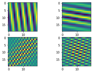
We can show the initial Gabor filters:

model.layers[0].show_filters()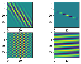

model.layers[2].show_filters()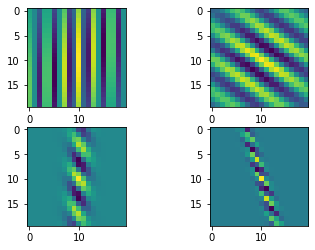

model.layers[4].show_filters()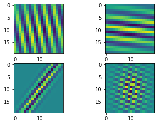

history = model.fit(X_train, Y_train, batch_size=128, epochs=2, validation_split=0.2)

Epoch 1/2

2022-09-20 12:47:43.857300: I tensorflow/stream_executor/cuda/cuda_dnn.cc:369] Loaded cuDNN version 8100
2022-09-20 12:47:44.350354: I tensorflow/core/platform/default/subprocess.cc:304] Start cannot spawn child process: No such file or directory

375/375 [==============================] - 51s 96ms/step - loss: 2.2364 - accuracy: 0.1946 - val_loss: 2.0396 - val_accuracy: 0.2788
Epoch 2/2
375/375 [==============================] - 36s 96ms/step - loss: 1.9230 - accuracy: 0.3473 - val_loss: 1.7555 - val_accuracy: 0.4182

Showing the training dynamics:

fig, axes = plt.subplots(1,2, figsize=(9,4))
axes[0].plot(history.history['loss'][1:], label="Train")
axes[0].plot(history.history['val_loss'][1:], label="Val")
axes[1].plot(history.history['accuracy'], label="Train")
axes[1].plot(history.history['val_accuracy'], label="Val")
plt.legend()
plt.show()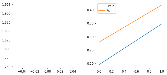

Calculate the metrics in the test set:

model.evaluate(X_test, Y_test, batch_size=128)

79/79 [==============================] - 0s 4ms/step - loss: 1.7527 - accuracy: 0.4212

[1.752727746963501, 0.4212000072002411]

We can visualize the gabor filters after the training process:

model.layers[0].show_filters()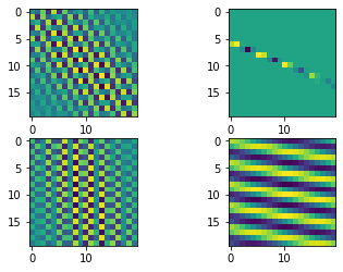

model.layers[2].show_filters()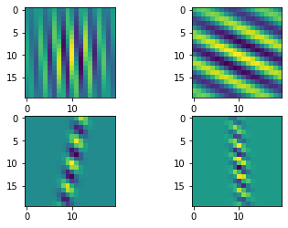

model.layers[4].show_filters()