Gabor layer experiment

In this quick experiment we will be training an MNIST classifier using GaborLayer layers.

Library importing

import numpy as np
import matplotlib.pyplot as plt
from einops import rearrange, repeat

import tensorflow as tf
from tensorflow.keras import layers
from tensorflow.keras.datasets import mnist

from flayers.layers import GaborLayer

Data loading

We will be using MNIST for a simple and quick test.

(X_train, Y_train), (X_test, Y_test) = mnist.load_data()

X_train = repeat(X_train, "b h w ->  b h w c", c=1)/255.0
X_test = repeat(X_test, "b h w ->  b h w c", c=1)/255.0

X_train.shape, Y_train.shape, X_test.shape, Y_test.shape

((60000, 28, 28, 1), (60000,), (10000, 28, 28, 1), (10000,))

Definition of simple model

n_gabors = 4
sigma_i = [0.1, 0.2]*2
sigma_j = [0.2, 0.1]*2
freq = [10, 10]*2
theta = [0, np.pi/2]*2
rot_theta = [0, 0]*2
sigma_theta = [0, 0]*2

model = tf.keras.Sequential([
    GaborLayer(n_gabors=n_gabors, size=20, imean=0.5, jmean=0.5, sigma_i=sigma_i, sigma_j=sigma_j, freq=freq, 
               theta=theta, rot_theta=rot_theta, sigma_theta=sigma_theta, fs=20, input_shape=(28,28,1)),
    layers.MaxPool2D(2),
    layers.GlobalAveragePooling2D(),
    layers.Dense(10, activation="softmax")
])
model.compile(optimizer="adam",
              loss="sparse_categorical_crossentropy",
              metrics=["accuracy"])
model.summary()

Model: "sequential_1"
_________________________________________________________________
Layer (type)                 Output Shape              Param #   
=================================================================
gabor_layer_1 (GaborLayer)   (None, 28, 28, 4)         1626      
_________________________________________________________________
max_pooling2d_1 (MaxPooling2 (None, 14, 14, 4)         0         
_________________________________________________________________
global_average_pooling2d_1 ( (None, 4)                 0         
_________________________________________________________________
dense_1 (Dense)              (None, 10)                50        
=================================================================
Total params: 1,676
Trainable params: 76
Non-trainable params: 1,600
_________________________________________________________________

We can show the initial Gabor filters:

model.layers[0].show_filters()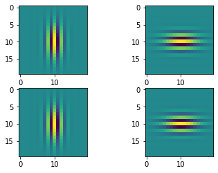

history = model.fit(X_train, Y_train, batch_size=128, epochs=1, validation_split=0.2)

375/375 [==============================] - 17s 33ms/step - loss: 2.2897 - accuracy: 0.1481 - val_loss: 2.2693 - val_accuracy: 0.1996

We can visualize the gabor filters after the training process:

model.layers[0].show_filters()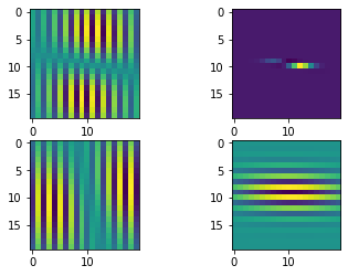

We can even check the atributes of the layer to inspect the change in the initial parameters:

model.layers[0].theta.numpy()*180/np.pi

array([-1.3238928, 90.20859  , -2.235493 , 88.482956 ], dtype=float32)

model.layers[0].rot_theta.numpy()*180/np.pi

array([-1.3243861 ,  0.27530777,  2.329611  , -1.5420123 ], dtype=float32)

model.layers[0].sigma_theta.numpy()*180/np.pi

array([-1.3520143, -4.6940336,  5.102634 , -1.5307682], dtype=float32)